Lecture_1 Linear Regression
pd.read_csv() 用法介绍 ,部分用法:
csv文件有表头并且是第一行,那么names和header都无需指定;
csv文件有表头、但表头不是第一行,可能从下面几行开始才是真正的表头和数据,这个时候指定header即可;
csv文件没有表头,全部是纯数据,那么我们可以通过names手动生成表头;
csv文件有表头、但是这个表头你不想用,这个时候同时指定names和header。先用header选出表头和数据,然后再用names将表头替换掉,就等价于将数据读取进来之后再对列名进行rename;
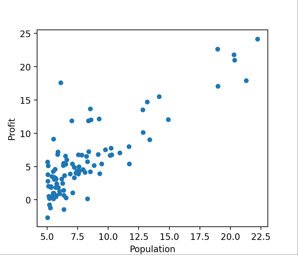
原始数据:
使用梯度下降 来实现线性回归,以最小化成本函数:
J ( θ ) = 1 2 m ∑ i = 1 m ( h θ ( x ( i ) ) − y ( i ) ) 2 J(\theta) = \frac{1}{2m}\sum_{i=1}^{m}(h_{\theta}(x^{(i)})-y^{(i)})^2
J ( θ ) = 2 m 1 i = 1 ∑ m ( h θ ( x ( i ) ) − y ( i ) ) 2
其中,h θ ( x ) = θ T X = θ 0 x 0 + θ 1 x 1 + … + θ n x n h_{\theta}(x) = \theta^{T}X=\theta_{0}x_0+\theta_1x_1+\ldots+\theta_nx_n h θ ( x ) = θ T X = θ 0 x 0 + θ 1 x 1 + … + θ n x n
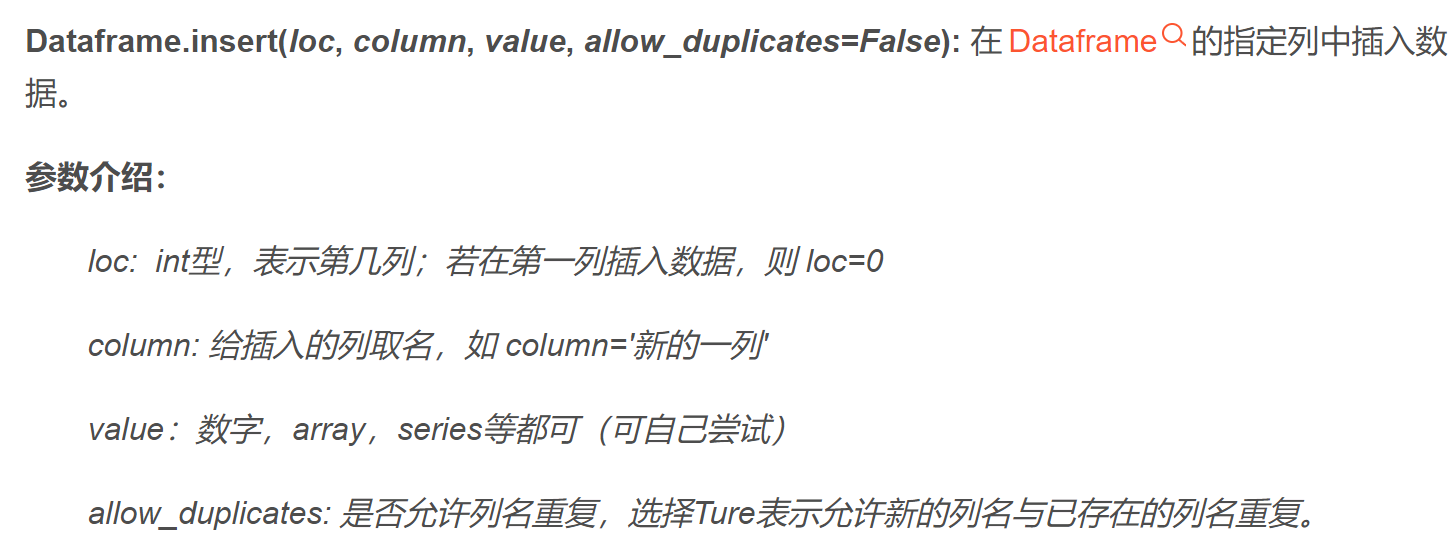
In [165 ]:data=pd.DataFrame(np.arange(16 ).reshape(4 ,4 ), columns=list ('abcd' )) In [166 ]:data Out[166 ]: a b c d 0 0 1 2 3 1 4 5 6 7 2 8 9 10 11 3 12 13 14 15 In [167 ]: data.insert(loc=0 ,column='haha' ,value=6 ) In [168 ]: data Out[168 ]: haha a b c d 0 6 0 1 2 3 1 6 4 5 6 7 2 6 8 9 10 11 3 6 12 13 14 15 In [169 ]: data.insert(loc=0 ,column='haha' ,value=6 ,allow_duplicates=True ) In [170 ]: data Out[170 ]: haha haha a b c d 0 6 6 0 1 2 3 1 6 6 4 5 6 7 2 6 6 8 9 10 11 3 6 6 12 13 14 15
尽量不要用np.matrix(),这会让事情变得更复杂,用np.to_numpy(),以及np.dot()
batch gradient descent(批量梯度下降)
θ ≔ θ j − ∂ ∂ θ j J ( θ ) \theta \coloneqq \theta_{j} - \frac{\partial}{\partial \theta_{j}}J(\theta)
θ : = θ j − ∂ θ j ∂ J ( θ )
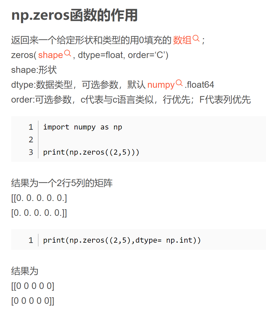
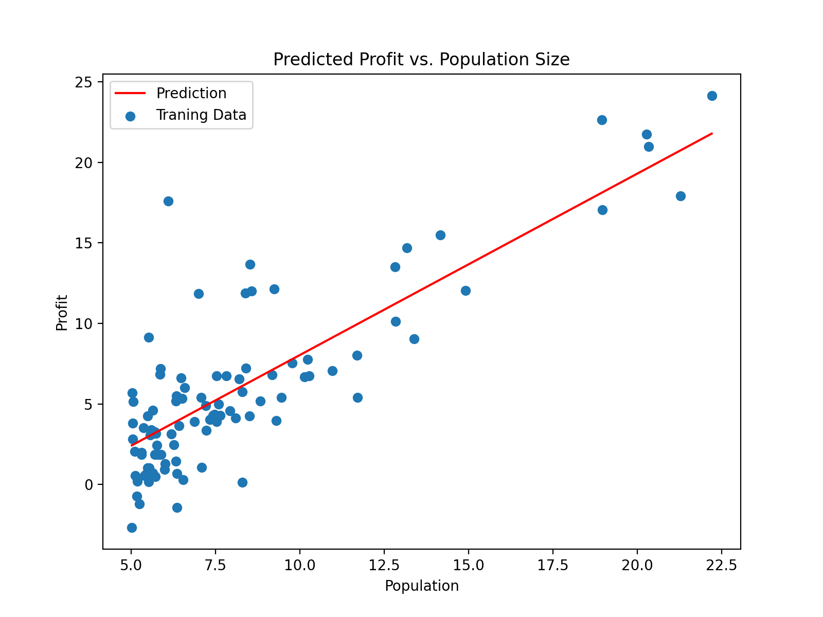
import numpy as npimport pandas as pdimport matplotlib.pyplot as pltpath = 'G:/machine learning/吴恩达/学习笔记/ex1data1.txt' data = pd.read_csv(path, header=None , names=['Population' , 'Profit' ]) data.plot(kind = 'scatter' , x = 'Population' , y = 'Profit' , figsize = (8 , 6 )) def computeCost (X, y, theta ): error = X.dot(theta) - y return (1 /2 / len (X)) * np.dot(error.T, error) data.insert(0 , 'Ones' , 1 ) cols = data.shape[1 ] X = data.iloc[:, 0 :cols-1 ] y = data.iloc[:, cols-1 :] X = X.to_numpy() y = y.to_numpy() theta = np.zeros((2 , 1 )) def gradientDescent (X, y, theta, alpha, iters ): temp = np.zeros(theta.shape) parameters = int (theta.ravel().shape[0 ]) cost = np.zeros(iters) for i in range (iters): error = (X.dot(theta) - y) for j in range (parameters): temp_X = np.array(X[:, j]).reshape(len (X), 1 ) term = np.dot(error.T, temp_X) temp[j, 0 ] = theta[j, 0 ] - ((alpha / len (X)) * term) theta = temp cost[i] = computeCost(X, y, theta) return theta, cost alpha = 0.01 iters = 1000 g, cost = gradientDescent(X, y, theta, alpha, iters) x = np.linspace(data.Population.min (), data.Population.max (), 100 ) f = g[0 , 0 ] + (g[1 , 0 ] * x) fig, ax = plt.subplots(figsize=(8 ,6 )) ax.plot(x, f, 'r' , label='Prediction' ) ax.scatter(data.Population, data.Profit, label='Traning Data' ) ax.legend(loc=2 ) ax.set_xlabel('Population' ) ax.set_ylabel('Profit' ) ax.set_title('Predicted Profit vs. Population Size' ) plt.show()
Linear Regression with multiple variables
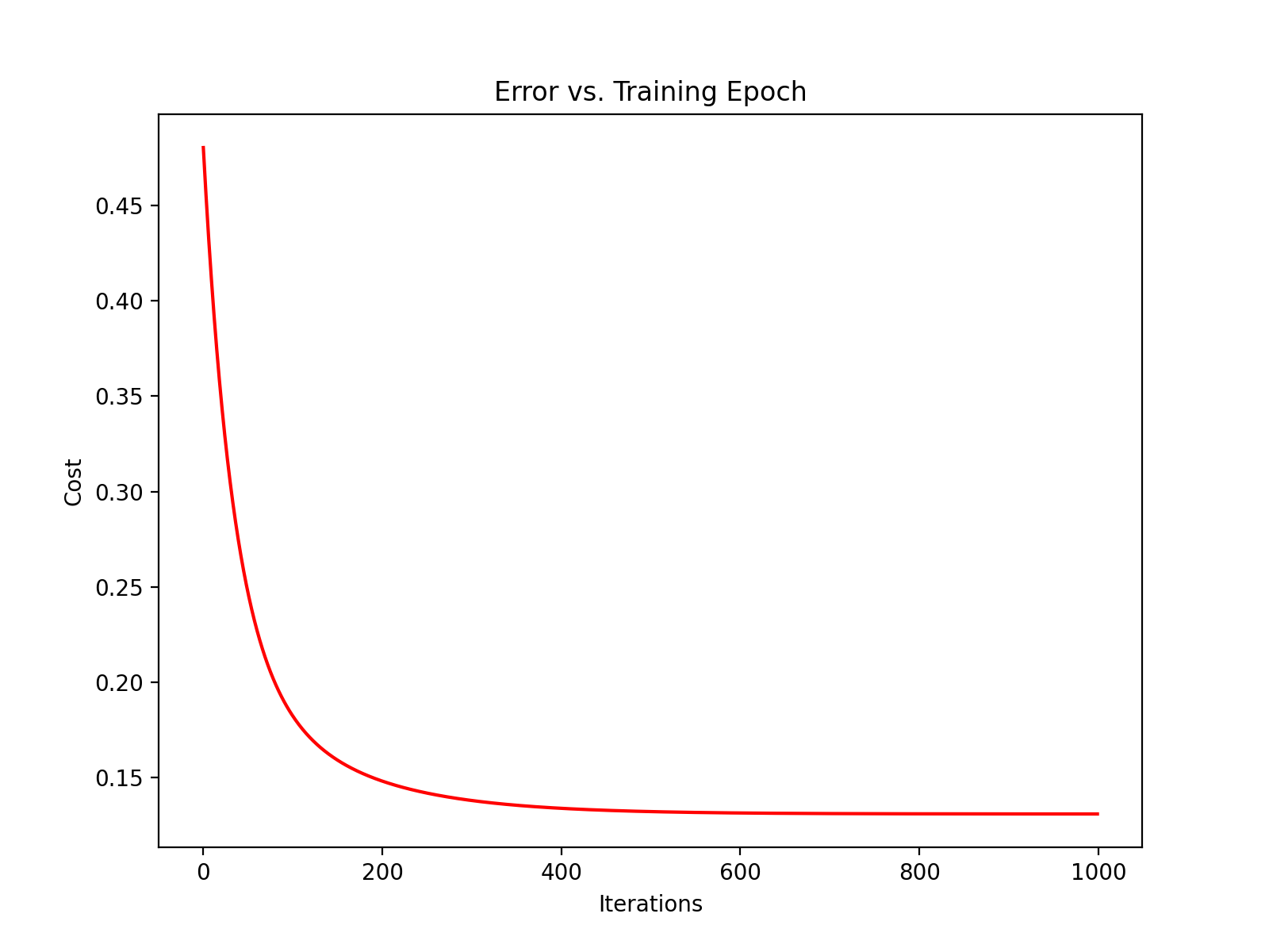
import numpy as npimport pandas as pdimport matplotlib.pyplot as pltpath = 'G:/machine learning/吴恩达/学习笔记/ex1data2.txt' data = pd.read_csv(path, header=None , names=['Size' , 'Bedrooms' , 'Price' ]) print(data.head()) data = (data - data.mean())/ data.std() print(data.head()) def computeCost (X, y, theta ): error = X.dot(theta) - y return (1 /2 / len (X)) * np.dot(error.T, error) data.insert(0 , 'Ones' , 1 ) cols = data.shape[1 ] X = data.iloc[:, 0 :cols-1 ] y = data.iloc[:, cols-1 :] X = X.to_numpy() y = y.to_numpy() theta = np.zeros((X.shape[1 ], 1 )) print(X.shape, y.shape, theta.shape) def gradientDescent (X, y, theta, alpha, iters ): temp = np.zeros(theta.shape) parameters = int (theta.ravel().shape[0 ]) cost = np.zeros(iters) for i in range (iters): error = (X.dot(theta) - y) for j in range (parameters): temp_X = np.array(X[:, j]).reshape(len (X), 1 ) term = np.dot(error.T, temp_X) temp[j, 0 ] = theta[j, 0 ] - ((alpha / len (X)) * term) theta = temp cost[i] = computeCost(X, y, theta) return theta, cost alpha = 0.01 iters = 1000 g, cost = gradientDescent(X, y, theta, alpha, iters) print(computeCost(X, y, g)) fig, ax = plt.subplots(figsize=(8 , 6 )) ax.plot(np.arange(iters), cost, 'r' ) ax.set_xlabel('Iterations' ) ax.set_ylabel('Cost' ) ax.set_title('Error vs. Training Epoch' ) plt.show()
使用scikit-learn的线性回归函数,而不是从头开始实现这些算法。 我们将scikit-learn的线性回归算法应用于第1部分的数据,并看看它的表现。
from sklearn import linear_modelmodel = linear_model.LinearRegression() model.fit(X, y) x = np.array(X[:, 1 ].A1) f = model.predict(X).flatten() fig, ax = plt.subplots(figsize=(8 ,6 )) ax.plot(x, f, 'r' , label='Prediction' ) ax.scatter(data.Population, data.Profit, label='Traning Data' ) ax.legend(loc=2 ) ax.set_xlabel('Population' ) ax.set_ylabel('Profit' ) ax.set_title('Predicted Profit vs. Population Size' ) plt.show()
正规方程是通过求解下面的方程来找出使得代价函数最小的参数的: ∂ ∂ θ j J ( θ j ) = 0 \frac{\partial}{\partial\theta_{j}}J(\theta_{j})=0 ∂ θ j ∂ J ( θ j ) = 0 X X X x 0 = 1 x_0 = 1 x 0 = 1 y y y θ = ( X T X ) − 1 X T y \theta = (X^{T}X)^{-1}X^{T}y θ = ( X T X ) − 1 X T y T T T − 1 -1 − 1 A = X T X A=X^{T}X A = X T X ( X T X ) − 1 = A − 1 (X^{T}X)^{-1} = A^{-1} ( X T X ) − 1 = A − 1
梯度下降与正规方程的比较:
梯度下降:需要选择学习率α,需要多次迭代,当特征数量n大时也能较好适用,适用于各种类型的模型
正规方程:不需要选择学习率α,一次计算得出,需要计算( X T X ) − 1 (X^{T}X)^{-1} ( X T X ) − 1 O ( n 3 ) O(n^{3}) O ( n 3 ) n n n