111
pandas.isin()函数使用方法,用于数据清洗,画出散点图如下:
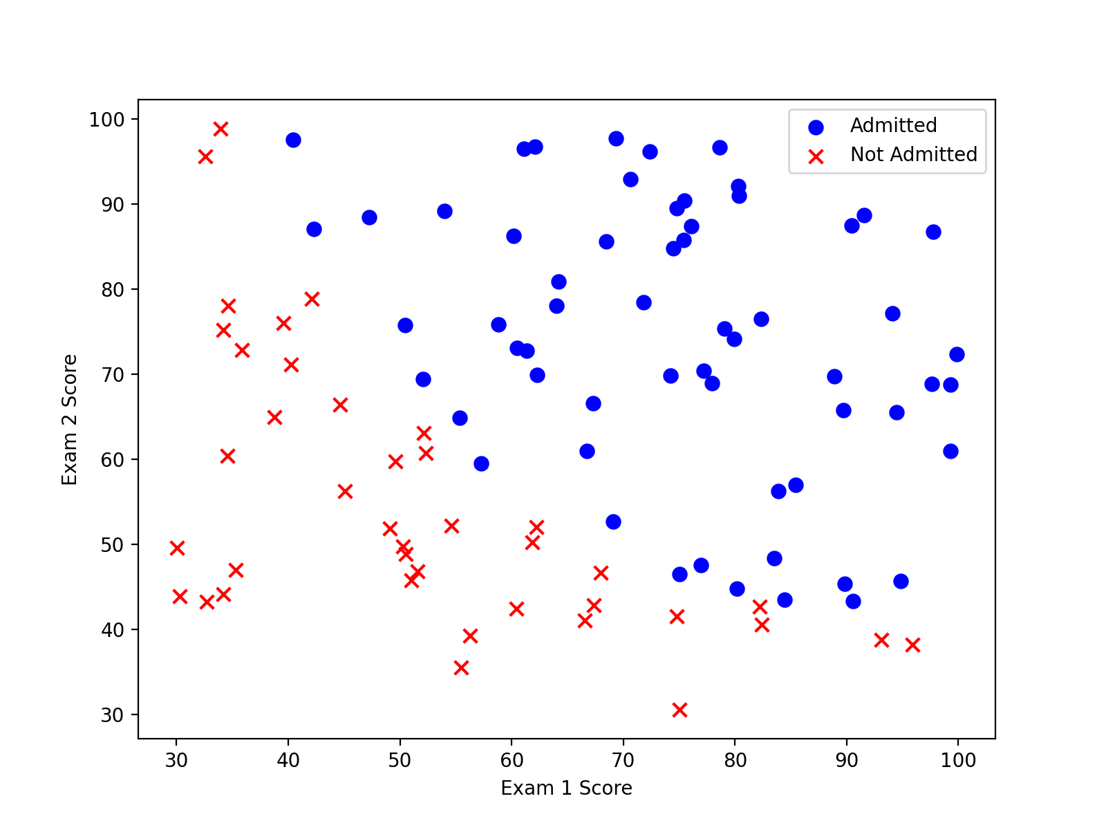
在两类数据中,很明显存在着一个明显的决策边界,可以采用逻辑回归的方式进行预测。
Sigmoid函数
g代表一个常用的逻辑函数(logistic function),为S型函数(sigmoid function),公式为:
g(z)=1+exp−z1
将g(z)与之前的线性方程相结合,得到逻辑回归的假设函数:
h(θj)=1+exp−θTX1
Logistic Regression 的代价函数为:
J(θ)=−m1i=1∑m[y(i)log(hθ(xi))+(1−y(i))log(1−hθ(xi))]
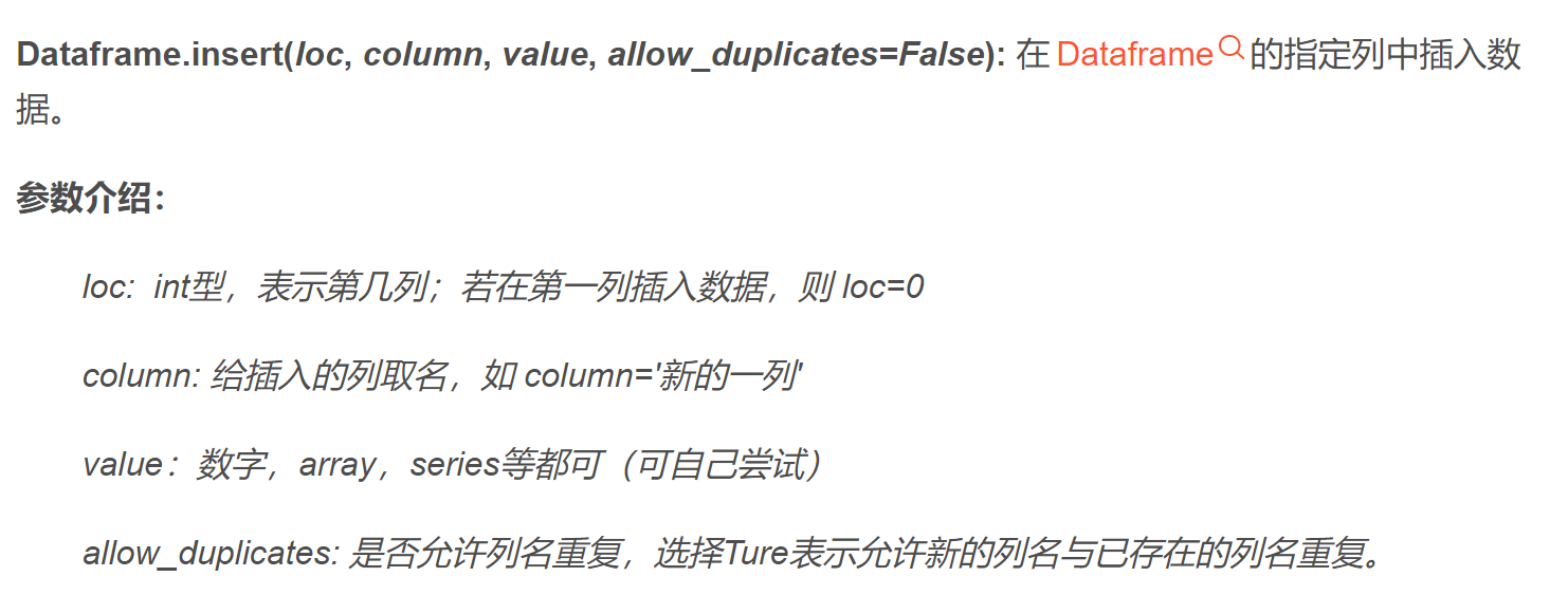
pandas.insert()用法详解,具体使用方法如下:
Gradient Descent(梯度下降)
∂θj∂J(θ)=m1i=1∑m(hθ(x(i))−y(i))xj(i)
注意,我们实际上没有在这个函数中执行梯度下降,我们仅仅在计算一个梯度步长。在练习中,一个称为“fminunc”的Octave函数是用来优化函数来计算成本和梯度参数。由于我们使用Python,我们可以用SciPy的“optimize”命名空间来做同样的事情。
Scipy’s truncated newton (TNC) 实现寻找最优参数,具体使用方法。
编写一个函数,用我们所学的参数theta来为数据集X输出预测。然后,我们可以使用这个函数来给我们的分类器的训练精度打分。 逻辑回归模型的假设函数:
hθ(x)=1+exp−θTX1
当hθ大于等于0.5时,预测 y=1;
当hθ小于0.5时,预测 y=0 ;
import numpy as np
import pandas as pd
import matplotlib.pyplot as plt
import scipy.optimize as opt
path = 'G:/machine learning/吴恩达/学习笔记/Lecture_2/ex2data1.txt'
data = pd.read_csv(path, header=None, names=['Exam 1', 'Exam 2', 'Admitted'])
print(data.head())
positive = data[data["Admitted"].isin([1])]
negative = data[data["Admitted"].isin([0])]
def sigmoid(z):
return 1 / (1 + np.exp(-z))
data.insert(0, 'Ones', 1)
cols = data.shape[1]
X = data.iloc[:, 0: cols-1]
y = data.iloc[:, cols-1: cols]
X = X.to_numpy()
y = y.to_numpy()
theta = np.zeros((X.shape[1], 1))
def computeCost(theta, X, y):
sum_1 = np.dot(np.log(sigmoid(np.dot(X, theta))).T, y)
sum_2 = np.dot(np.log(1- sigmoid(np.dot(X, theta))).T, 1-y)
return -1/len(X) * (sum_1 + sum_2)
print(computeCost(theta, X, y))
def gradientdescent(theta, X, y):
theta = theta.reshape(theta.shape[0], 1)
error = (sigmoid(np.dot(X, theta)) - y)
grad = np.zeros(theta.shape)
for j in range(X.shape[1]):
temp_X = np.array(X[:,j]).reshape((len(X), 1))
grad[j,0] = (1 /len(X) * np.dot(error.T, temp_X))[0,0]
return grad
result = opt.fmin_tnc(func=computeCost, x0=theta, fprime=gradientdescent, args=(X, y))
def predict(X, theta):
predict_value = sigmoid(np.dot(X, theta))
return [1 if each_predict_value >= 0.5 else 0 for each_predict_value in predict_value]
predictions = predict(X, np.array(result[0]))
correct = [1 if ((a == 1 and b == 1) or (a == 0 and b == 0)) else 0 for (a, b) in zip(predictions, y)]
accuracy = (sum(map(int, correct)) % len(correct))
print ('accuracy = {0}%'.format(accuracy))
|
Regularized Logistic Regression(正则化逻辑回归)
简而言之,正则化是成本函数中的一个术语,它使算法更倾向于“更简单”的模型(在这种情况下,模型将更小的系数)。这个理论助于减少过拟合,提高模型的泛化能力。
设想你是工厂的生产主管,你有一些芯片在两次测试中的测试结果。对于这两次测试,你想决定是否芯片要被接受或抛弃。为了帮助你做出艰难的决定,你拥有过去芯片的测试数据集,从其中你可以构建一个逻辑回归模型。
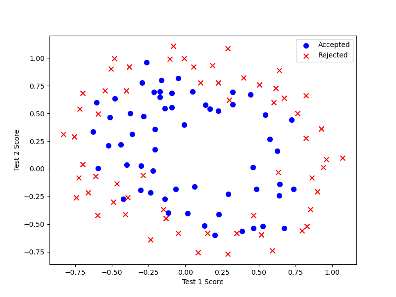
这个数据看起来可比前一次的复杂得多。特别地,其中没有线性决策界限,来良好的分开两类数据。一个方法是用像逻辑回归这样的线性技术来构造从原始特征的多项式中得到的特征。通过创建一组多项式特征入手。
pandas.drop()函数使用方法。
对于正则化后的代价函数,应该更正为:
J(θ)=m1i=1∑m[−y(i)log(hθ(x(i)))−(1−y(i))log(1−hθ(x(i)))]+2mλj=1∑nθj2
该代价函数中,加入了学习率这个参数,这是超参数,用来控制正则化项。下面是正则化梯度函数:
Repeat until convergence{θ0:=θ0−am1i=1∑m[hθ(x(i))−y(i)]x0(i)θj:=θj−am1i=1∑m[hθ(x(i))−y(i)]xj(i)+mλθj}Repeat
对上面的算法中 j=1,2,...,n 时的更新式子进行调整可得:
θj:=θj(1−amλ)−am1i=1∑m(hθ(x(i))−y(i))xj(i)
虽然我们实现了这些算法,值得注意的是,我们还可以使用高级Python库像scikit-learn来解决这个问题。
import numpy as np
import pandas as pd
import matplotlib.pyplot as plt
import scipy.optimize as opt
path = 'G:/machine learning/吴恩达/学习笔记/Lecture_2/ex2data2.txt'
data = pd.read_csv(path, header=None, names=['Test 1', 'Test 2', 'Accepted'])
positive = data[data["Accepted"].isin([1])]
negative = data[data["Accepted"].isin([0])]
def sigmoid(z):
return 1 / (1 + np.exp(-z))
def computeCost(theta, X, y, learningRate):
theta = theta.reshape((theta.shape[0], 1))
sum_1 = np.dot(np.log(sigmoid(np.dot(X, theta))).T, y)
sum_2 = np.dot(np.log(1- sigmoid(np.dot(X, theta))).T, 1-y)
reg = (learningRate/(2 * len(X))) * np.sum(np.power(theta[1:, :], 2))
return -1/len(X) * (sum_1 + sum_2) + reg
def gradient(theta, X, y, learningRate):
theta = theta.reshape(theta.shape[0], 1)
error = (sigmoid(np.dot(X, theta)) - y)
grad = np.zeros(theta.shape)
for j in range(X.shape[1]):
temp_X = np.array(X[:,j]).reshape((len(X), 1))
if (j == 0):
grad[j,0] = (1 /len(X) * np.dot(error.T, temp_X))[0,0]
else:
grad[j,0] = (1 /len(X) * np.dot(error.T, temp_X))[0,0] + (learningRate / len(X)) * theta[j, :]
return grad
def predict(X, theta):
theta = theta.reshape(theta.shape[0], 1)
predict_value = sigmoid(np.dot(X, theta))
return [1 if each_predict_value >= 0.5 else 0 for each_predict_value in predict_value]
degree = 5
x1 = data['Test 1']
x2 = data['Test 2']
data.insert(3, 'Ones', 1)
for i in range(1, degree):
for j in range(0, i):
data['F' + str(i) + str(j)] = np.power(x1, i-j) * np.power(x2, j)
data.drop('Test 1', axis=1, inplace=True)
data.drop('Test 2', axis=1, inplace=True)
cols = data.shape[1]
X = data.iloc[:,1:cols]
y = data.iloc[:,0:1]
X = X.to_numpy()
y = y.to_numpy()
theta = np.zeros((X.shape[1], 1))
learningrate = 1
result = opt.fmin_tnc(func=computeCost, x0=theta, fprime=gradient, args=(X, y, learningrate))
print(result)
predictions = predict(X, np.array(result[0]))
correct = [1 if ((a == 1 and b == 1) or (a == 0 and b == 0)) else 0 for (a, b) in zip(predictions, y)]
accuracy = (sum(map(int, correct)) / len(correct))
print ('accuracy = {0}%'.format(100 * accuracy))
|
可以使用高级Python库像scikit-learn来解决这个问题
from sklearn import linear_model
model = linear_model.LogisticRegression(penalty='l2', C=1.0)
model.fit(X, y.ravel())
print(model.score(X, y))
|