TUB_Course_Event camera 笔记总结

这里先附上课程的B站链接🔗[https://www.bilibili.com/video/BV1Zr4y1N7Vu?p=9&vd_source=69422cf7939fd0849b3b4cee11e7525c]，是从原课程班运过来的，主要没有翻译，其实看起来很难受😭，而且事件相机很多材料其实都是英文的，读起来就很费劲，希望自己能慢慢成长克服吧

Week2-Event representation

课程目标：

• 熟悉事件相机处理数据方式
• 练习将事件数据转换到“image-like”表达方式，包括grid-based, array-based
• 找到最佳（最合适）的事件数据表达方式

这里课程采用的是来自于Event Camera Dataset and Simulator (IJRR’17)的数据集->slider_depth，这里数据是txt格式，容易可视化并且数据大小很小；

在之前的学习中应该了解过，事件数据主要产生的有四类数据，分别是$(t,x,y,p)$，分别包含时间戳、空间信息和光亮变化信息；如何处理并可视化该数据是本节课的重点；

预先包引用

import os
import numpy as np
from matplotlib import pyplot as plt

事件数据提取

# Simple codre. There may be more efficient ways.
def extract_data(filename):
    infile = open(filename, 'r')
    timestamp = []
    x = []
    y = []
    pol = []
    for line in infile:
        words = line.split()
        timestamp.append(float(words[0]))
        x.append(int(words[1]))
        y.append(int(words[2]))
        pol.append(int(words[3]))
    infile.close()
    return timestamp,x,y,pol

filename_sub = 'slider_depth/events_chunk.txt'
# Call the function to read data    
timestamp, x, y, pol = extract_data(filename_sub)

img_size = (180, 240)

Image-like (2D grid) representation

Histograms of events (Event count)

在一定的事件数量下，将事件进行叠加，其实就是accumulating event polarities

# Accumulating the event polarities

num_event = 5000 #define the event numbers

img = np.zeros(img_size)

for each_event in range(num_event):
    img[y[each_event],x[each_event]] += (2*pol[each_event]) - 1 #convert the polarity bit from {0,1} to {-1,+1}

fig = plt.figure()
fig.suptitle('Balance of event polarities')
maxabsval = np.amax(np.abs(img)) #find the max abs value in the metrix img
plt.imshow(img, cmap='gray', clim=(-maxabsval, maxabsval)) #cmap: colormap clim: colorlimit
plt.xlabel("x [pixels]")
plt.ylabel("y [pixels]")
plt.colorbar()
plt.show()

上面的这个是采用的是gray灰度映射，这里如果换一种映射方式，可能会更清晰（也许吧，官方文档中写的是pseudocolor[https://en.wikipedia.org/wiki/False_color]

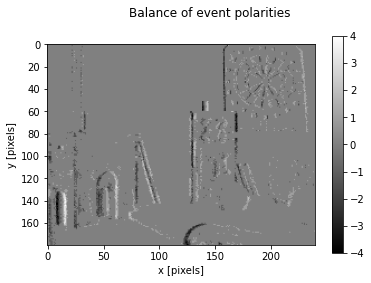
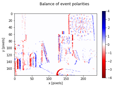
# Same plot as above, but changing the color map
fig = plt.figure()
fig.suptitle('Balance of event polarities')
maxabsval = np.amax(np.abs(img))
plt.imshow(img, cmap='seismic_r', clim=(-maxabsval,maxabsval))
plt.xlabel("x [pixels]")
plt.ylabel("y [pixels]")
plt.colorbar()
plt.show()

如果不对事件进行count，直接采用最后一个事件来可视化，其实就是这里称的ternary image

# Time Surface (or time map, or SAE="Surface of Active Events")
num_event = len(timestamp)
print("Time surface: numevents = ", num_event)

sae_pos = np.zeros(img_size, np.float32)
sae_neg = np.zeros(img_size, np.float32)
time_ref = timestamp[-1] # time of the last event in the packet
tau = 0.03 # decay parameter (in seconds) depends on motion of the scene

for each_event in range (num_event):
    if pol[each_event] > 0:
        sae_pos[y[each_event], x[each_event]] = np.exp(-(time_ref - timestamp[each_event])/tau)
    else:
        sae_neg[y[each_event], x[each_event]] = np.exp(-(time_ref - timestamp[each_event])/tau)

#plot SAE_positive
fig = plt.figure()
fig.suptitle('Time surface (exp decay) of positive polarities')
plt.imshow(sae_pos)
plt.xlabel("x [pixels]")
plt.ylabel("y [pixels]")
plt.colorbar()
plt.show()

#plot SAE_negative
fig = plt.figure()
fig.suptitle('Time surface (exp decay) of negative polarities')
plt.imshow(sae_neg)
plt.xlabel("x [pixels]")
plt.ylabel("y [pixels]")
plt.colorbar()
plt.show()

Image of timstampes

另一种有效的表达形式，不计算每个像素的事件数量，而是展示每个像素的时间戳，包括最新的事件的时间戳，平均时间戳，或者一种带有指数衰减的时间戳，也称为“time surfaces”、“time maps”、“surface of active events”；

带有指数衰减的Time maps

这个表达方式由 2015 PAMI paper HOTS, Fig.2提出，公式表达为：

$$image(x,y;t)=exp(-|t-T(x,y)|/\tau)$$

$\tau$是一个可调参数，依赖于场景中的运动；

# Time Surface (or time map, or SAE="Surface of Active Events")
num_event = len(timestamp)
print("Time surface: numevents = ", num_event)

img = np.zeros(img_size, np.float32)
time_ref = timestamp[-1] # time of the last event in the packet
tau = 0.03 # decay parameter (in seconds) depends on motion of the scene

for each_event in range (num_event):
    img[y[each_event], x[each_event]] = np.exp(-(time_ref - timestamp[each_event])/tau)

#plot SAE
fig = plt.figure()
fig.suptitle('Time surface (exp decay). Both polarities')
plt.imshow(img)
plt.xlabel("x [pixels]")
plt.ylabel("y [pixels]")
plt.colorbar()
plt.show()

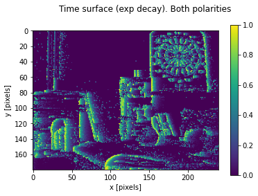
# Time Surface (or time map, or SAE="Surface of Active Events")
num_event = len(timestamp)
print("Time surface: numevents = ", num_event)

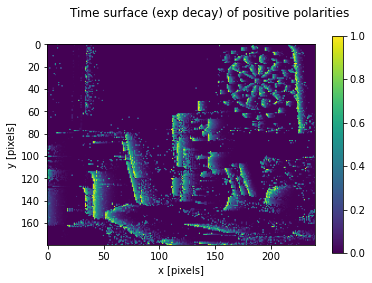
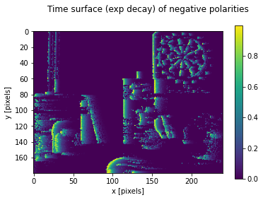
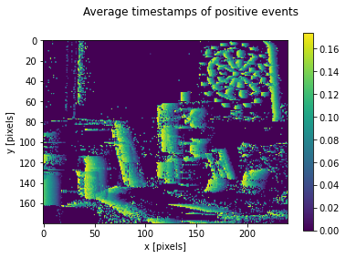
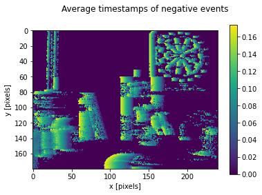
sae_pos = np.zeros(img_size, np.float32)
sae_neg = np.zeros(img_size, np.float32)
time_ref = timestamp[-1] # time of the last event in the packet
tau = 0.03 # decay parameter (in seconds) depends on motion of the scene

for each_event in range (num_event):
    if pol[each_event] > 0:
        sae_pos[y[each_event], x[each_event]] = np.exp(-(time_ref - timestamp[each_event])/tau)
    else:
        sae_neg[y[each_event], x[each_event]] = np.exp(-(time_ref - timestamp[each_event])/tau)

#plot SAE_positive
fig = plt.figure()
fig.suptitle('Time surface (exp decay) of positive polarities')
plt.imshow(sae_pos)
plt.xlabel("x [pixels]")
plt.ylabel("y [pixels]")
plt.colorbar()
plt.show()

#plot SAE_negative
fig = plt.figure()
fig.suptitle('Time surface (exp decay) of negative polarities')
plt.imshow(sae_neg)
plt.xlabel("x [pixels]")
plt.ylabel("y [pixels]")
plt.colorbar()
plt.show()

Average timestamp images

计算几毫米之内，每个像素下时间戳的平均值；这里没有指数衰减，仅仅是平均值

#Average timestamp per pixel
sae = np.zeros(img_size, np.float32)
count = np.zeros(img_size, np.int32)

for each_event in range(num_event):
    sae[y[each_event], x[each_event]] += timestamp[each_event]
    count[y[each_event], x[each_event]] += 1

count[count < 1] = 1 # avoid division by zero
sae = sae / count # average

#plot 
fig = plt.figure()
fig.suptitle('Average timestamps regardless of polarity')
plt.imshow(sae)
plt.xlabel("x [pixels]")
plt.ylabel("y [pixels]")
plt.colorbar()
plt.show()

# %% Average timestamp per pixel. Separate by polarity
sae_pos = np.zeros(img_size, np.float32)
sae_neg = np.zeros(img_size, np.float32)
count_pos = np.zeros(img_size, np.int32)
count_neg = np.zeros(img_size, np.int32)
for i in range(num_event):
    if (pol[i] > 0):
        sae_pos[y[i],x[i]] += timestamp[i]
        count_pos[y[i],x[i]] += 1
    else:
        sae_neg[y[i],x[i]] += timestamp[i]
        count_neg[y[i],x[i]] += 1
    
# Compute per-pixel average if count at the pixel is >1
count_pos [count_pos < 1] = 1;  sae_pos = sae_pos / count_pos
count_neg [count_neg < 1] = 1;  sae_neg = sae_neg / count_neg

fig = plt.figure()
fig.suptitle('Average timestamps of positive events')
plt.imshow(sae_pos)
plt.xlabel("x [pixels]")
plt.ylabel("y [pixels]")
plt.colorbar()
plt.show()

fig = plt.figure()
fig.suptitle('Average timestamps of negative events')
plt.imshow(sae_neg)
plt.xlabel("x [pixels]")
plt.ylabel("y [pixels]")
plt.colorbar()
plt.show()

Space-time plots

定义一定的事件数量，可视化固定数量下 x，y，t的三维视图，对所有亮度变化做出反应，3D plot，可以切换不同视角

# %% 3D plot 
# Time axis in horizontal position

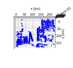
m = 2000 # Number of points to plot
print("Space-time plot and movie: numevents = ", m)

# Plot without polarity
fig = plt.figure()
ax = fig.add_subplot(111, projection='3d')
#ax.set_aspect('equal') # only works for time in Z axis
ax.scatter(x[:m], timestamp[:m], y[:m], marker='.', c='b')
ax.set_xlabel('x [pix]')
ax.set_ylabel('time [s]')
ax.set_zlabel('y [pix] ')
ax.view_init(azim=-90, elev=-180) # Change viewpoint with the mouse, for example
plt.show()

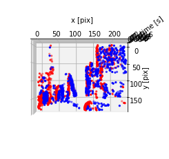
# %% Plot each polarity with a different color (red / blue)
idx_pos = np.asarray(pol[:m]) > 0 # the index of positive event
idx_neg = np.logical_not(idx_pos) # the index of negative event
xnp = np.asarray(x[:m])
ynp = np.asarray(y[:m])
tnp = np.asarray(timestamp[:m])
fig = plt.figure()
ax = fig.add_subplot(111, projection='3d')
ax.scatter(xnp[idx_pos], tnp[idx_pos], ynp[idx_pos], marker='.', c='b')
ax.scatter(xnp[idx_neg], tnp[idx_neg], ynp[idx_neg], marker='.', c='r')
ax.set(xlabel='x [pix]', ylabel='time [s]', zlabel='y [pix]')
ax.view_init(azim=-90, elev=-180)
plt.show()

Voxel grid representation

Regular histogram

这个表达方式主要是由Alex Zhu’s paper提出的，用于作光流估计的相关工作，课程中没有给出对应的数学公式，所以对代码的理解会存在问题，这里引用一下论文中的数学公式来有助于理解数据的表达方式：

$$\begin{align} t^*_{i} &= (B-1)(t_{i}-t_{0})/(t_{N-1}-t_{0}) \\ V(x,y,t) &= \sum_{i} p_{i}max(0,1-|x-x_{i}|)max(0,1-|y-y_{i}|)max(0,1-|t-t^*_{i}|) \end{align}$$

这里简单说一下我自己的理解再放代码，首先$t^*_{i}$是将事件的时间戳缩放到[0,B-1]的范围内，然后计算(x,y)位置像素范围内 事件时间戳的数量叠加，以此来表达事件数据；

后面的工作我简单写一下，考虑到每个像素所作的光流估计：$u(x,y),v(x,y)$，如何去表示光流估计后的坐标位置呢？经过scale的事件：$\{(x_{i},y_{i},t^*_{i},p_i)\}_{i=1,…,N}$，propagate，传播到一个时刻$t'$时的位置：

$$\left(\begin{array}{l} x_{i}^{\prime} \\ y_{i}^{\prime} \end{array}\right)=\left(\begin{array}{l} x_{i} \\ y_{i} \end{array}\right)+\left(t^{\prime}-t_{i}^{*}\right)\left(\begin{array}{c} u\left(x_{i}, y_{i}\right) \\ v\left(x_{i}, y_{i}\right) \end{array}\right)$$

最后按照不同极性，生成两个图像$T_{+}$和$T_{-}$，记录的是每个像素的平均时间戳信息，但是这里作者强调了采用的像素坐标的插值而不是四舍五入的差值方法，结果很不相同，也许之后可以学习一下。

$$T_{\{+,-\}}\left(x, y, t^{\prime}\right)=\frac{\sum_{i} \max \left(0,1-\left|x-x_{i}^{\prime}\right|\right) \max \left(0,1-\left|y-y_{i}^{\prime}\right|\right) t_{i}}{N(x, y)}$$

Loss 是用以下计算的：

$$\mathcal{L}_{\mathrm{time}}\left(t^{\prime}\right)=\sum_{x} \sum_{y} T_{+}(x, y)^{2}+T_{-}(x, y)^{2}$$

# %% Voxel grid

num_bins = 5 
print("Number of time bins = ", num_bins)

t_max = np.amax(np.asarray(timestamp[:m]))
t_min = np.amin(np.asarray(timestamp[:m]))
t_range = t_max - t_min
dt_bin = t_range / num_bins # size of the time bins (bins)
t_edges = np.linspace(t_min,t_max,num_bins+1) # Boundaries of the bins

# Compute 3D histogram of events manually with a loop
# ("Zero-th order or nearest neighbor voting")
hist3d = np.zeros(img.shape+(num_bins,), np.int)
for ii in xrange(m):
    idx_t = int( (timestamp[ii]-t_min) / dt_bin )
    if idx_t >= num_bins:
        idx_t = num_bins-1 # only one element (the last one)
    hist3d[y[ii],x[ii],idx_t] += 1

# Checks:
print("hist3d")
print(hist3d.shape)
print(np.sum(hist3d)) # This should equal the number of votes

# %% Compute 3D histogram of events using numpy function histogramdd
# https://docs.scipy.org/doc/numpy/reference/generated/numpy.histogramdd.html#numpy.histogramdd

# Specify bin edges in each dimension
bin_edges = (np.linspace(0,img_size[0],img_size[0]+1), 
             np.linspace(0,img_size[1],img_size[1]+1), t_edges)
yxt = np.transpose(np.array([y[:m], x[:m], timestamp[:m]]))
hist3dd, edges = np.histogramdd(yxt, bins=bin_edges)

# Checks
print("\nhist3dd")
print("min = ", np.min(hist3dd))
print("max = ", np.max(hist3dd))
print (np.sum(hist3dd))
print (np.linalg.norm( hist3dd - hist3d)) # Check: zero if both histograms are equal 三维向量求范数
print("Ratio of occupied bins = ", np.sum(hist3dd > 0) / float(np.prod(hist3dd.shape)) )


# Plot of the 3D histogram. Empty cells are transparent (not displayed)
# Example: https://matplotlib.org/3.1.1/gallery/mplot3d/voxels_rgb.html#sphx-glr-gallery-mplot3d-voxels-rgb-py

fig = plt.figure()
fig.suptitle('3D histogram (voxel grid), zero-th order voting')
ax = fig.gca(projection='3d')
# prepare some coordinates
r, g, b = np.indices((img_size[0]+1,img_size[1]+1,num_bins+1))
ax.voxels(g,b,r, hist3d) # No need to swap the data to plot with reordered axes
ax.set(xlabel='x', ylabel='time bin', zlabel='y')
ax.view_init(azim=-90, elev=-180) # edge-on, along time axis
#ax.view_init(azim=-63, elev=-145) # oblique viewpoint
plt.show()

下面是一些关于插值的表达方法，这里不作具体的解释了，仅仅贴一下代码吧

# %% Compute interpolated 3D histogram (voxel grid)
hist3d_interp = np.zeros(img.shape+(num_bins,), np.float64)
for ii in xrange(m-1):
    tn = (timestamp[ii] - t_min) / dt_bin # normalized time, in [0,num_bins]
    ti = np.floor(tn-0.5) # index of the left bin 
    dt = (tn-0.5) - ti    # delta fraction
    # Voting on two adjacent bins
    if ti >=0 :
        hist3d_interp[y[ii],x[ii],int(ti)  ] += 1. - dt
    if ti < num_bins-1 :
        hist3d_interp[y[ii],x[ii],int(ti)+1] += dt

# Checks
print("\nhist3d_interp")
print("min = ", np.min(hist3d_interp))
print("max = ", np.max(hist3d_interp))
print np.sum(hist3d_interp)
# Some votes are lost because of the missing last layer
print np.linalg.norm( hist3d - hist3d_interp)
print("Ratio of occupied bins = ", np.sum(hist3d_interp > 0) / float(np.prod(hist3d_interp.shape)) )

# Plot voxel grid
colors = np.zeros(hist3d_interp.shape + (3,))
tmp = hist3d_interp/np.amax(hist3d_interp) # normalize in [0,1]
colors[..., 0] = tmp
colors[..., 1] = tmp
colors[..., 2] = tmp

fig = plt.figure()
fig.suptitle('Interpolated 3D histogram (voxel grid)')
ax = fig.gca(projection='3d')
ax.voxels(g,b,r, hist3d_interp, facecolors=colors)
ax.set(xlabel='x', ylabel='time bin', zlabel='y')
ax.view_init(azim=-63, elev=-145)
plt.show()

# %% A different visualization viewpoint
ax.view_init(azim=-90, elev=-180) # edge-on, along time axis
plt.show()

# %% Compute interpolated 3D histogram (voxel grid) using polarity
hist3d_interp_pol = np.zeros(img.shape+(num_bins,), np.float64)
for ii in xrange(m-1):
    tn = (timestamp[ii] - t_min) / dt_bin # normalized time, in [0,num_bins]
    ti = np.floor(tn-0.5) # index of the left bin
    dt = (tn-0.5) - ti    # delta fraction
    # Voting on two adjacent bins
    if ti >=0 :
        hist3d_interp_pol[y[ii],x[ii],int(ti)  ] += (1. - dt) * (2*pol[ii]-1)
    if ti < num_bins-1 :
        hist3d_interp_pol[y[ii],x[ii],int(ti)+1] += dt * (2*pol[ii]-1)

# Checks
# Some votes are lost because of the missing last layer
print("\nhist3d_interp_pol")
print("min = ", np.min(hist3d_interp_pol))
print("max = ", np.max(hist3d_interp_pol))
print np.sum(np.abs(hist3d_interp_pol))
print("Ratio of occupied bins = ", np.sum(np.abs(hist3d_interp_pol) > 0) / float(np.prod(hist3d_interp_pol.shape)) )

# Plot interpolated voxel grid using polarity
# Normalize the symmetric range to [0,1]
maxabsval = np.amax(np.abs(hist3d_interp_pol))
colors = np.zeros(hist3d_interp_pol.shape + (3,))
tmp = (hist3d_interp_pol + maxabsval)/(2*maxabsval)
colors[..., 0] = tmp
colors[..., 1] = tmp
colors[..., 2] = tmp

fig = plt.figure()
fig.suptitle('Interpolated 3D histogram (voxel grid), including polarity')
ax = fig.gca(projection='3d')
ax.voxels(g,b,r, hist3d_interp_pol, facecolors=colors)
ax.set(xlabel='x', ylabel='time bin', zlabel='y')
ax.view_init(azim=-63, elev=-145)
plt.show()

# %% Better visualization viewpoint to see positive and negative edges
ax.view_init(azim=-90, elev=-180) # edge-on, along time axis
plt.show()